Approaches to Spatial Data Mining
Luboš Popelínský
Faculty of Informatics, Masaryk University Brno
Czech Republic
Email: popel@fi.muni.cz
Abstract
We presents some approaches for mining spatial data both from relational and object-oriented databases that represent the first steps in that area. Most of spatial mining algorithms must employ some kind of neighbourhood relationships. We describe an extension of spatial (relational) database management for processing of spatial neighbourhood relations. This proposal allows an efficient integration of mining algorithms with the spatial database management system.GeoMiner system for mining in relational spatial database system is briefly described. Than two approaches to knowledge discovery in spatial object-oriented databases are introduced. They both bring an extension of spatial mining inductive languages, the first one by means of fuzzy set theory, the second one by means of inductive logic programming.
Abstrakt
Objevování znalostí v databázích je def
inuje jako hledání znalosti skryté v uložených datech. Pojednáváme o některých přístupech k dolování prostorových dat jak v prostředí relačních tak objektových databází. Tyto algoritmy využívají většinou někrteré z relací sousednosti. Popisujeme rozšíření relačního DBMS, které umožňuje efektivně integrovat dolovací algoritmy a systém GeoMiner pro dolování v prostorové relační databázi. Uvádíme dva přístupy k dolování v objektových databázích, které rozšiřují dolovací jazyky pomocí prostředků fuzzy množin a induktivního logického programování.1. Introduction
The growth of the number and the size of spatial databases exceeds human capabilities to analyse those databases in order to find implicit knowledge hidden in the data. That's why any kind of software support would be welcome. Knowledge discovery in databases (KDD) [1,6,18] has been characterised as an extraction of such knowledge from databases. Main tasks when mining geographic data [14] are, among others, understanding data, discovering relationship as well as (re)organising geographic databases. In spatial databases typical tasks for KDD should be clustering of similar objects, a description of a class of objects (e.g. by a subset of its attributes), finding associations between both spatial and non-spatial attributes or e.g. deviation of non-spatial attributes with respect to the spatial ones [5].
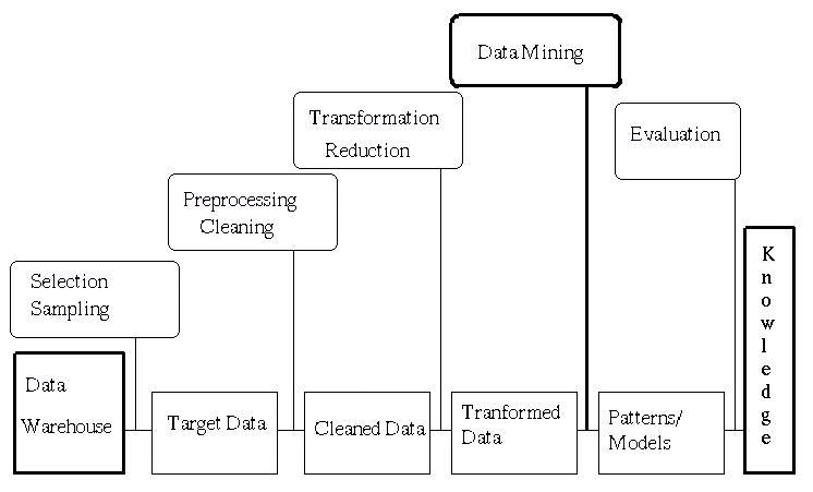
The whole process of KDD is on the Pic. 1. In this paper we focus only in the heart of the process, data mining. Data mining tasks can be divided into following 4 generic tasks. Class identification groups database objects into similarity subclasses. Classification results in a description of a given portion of a database in more compact way (e.g. by finding typical individuals or, more often, by describing the data by means of logic). Dependency analysis allows to predict the values of some attributes if knowing the values of others. Deviation detection discovers deviations from the expectations.
2. Knowledge Discovery in Spatial Data
The discovery process needs to be supported by the database management system itself [12]. There are more reasons that support that statement. First, knowledge discovery is an incremental process from a point of view a user; when a piece of knowledge is found usually its refinement and/or explanation is asked afterwards. Discovery algorithms should be from implementation point of view incremental as well. When updating the database, it is not optimal to run a mining algorithm again on the whole database. Better solutions would be to modify the mined result with respect to that updates. Some first ideas how to adapt classical database management systems for discovery tasks can be found in [12]. We will illustrate main topics of spatial mining by an example [4]. In can be proved that central places (e.g. central cities) may influence the values of some attributes of their neighbourhood such that they decrease with increasing distance. If we are interested e.g. in trends of unemployment, we first look for a minimum of the relevant attributes and then built the initial hypothesis, e.g.
when moving away from Munich
the unemployment rate increases
when moving away from Munich towards the north east
the unemployment rate decreases
when moving away from Munich towards the airport
the unemployment rate decreases
3. Mining in Relational Databases
In [4], a set of basic operations for spatial data mining is introduced that allows to express many existing mining algorithms. We give a brief overview of that approach in this section. We follows with a description of GeoMiner [11] system for mining in relational databases.
3.1. Basic Operations for Spatial Mining
Most of spatial mining algorithms must employ some kind of neighbourhood relationships. In [4] an extension of spatial database management system is proposed for processing of spatial neighbourhood relations. It was shown that four the most common mining algorithms can be expressed in terms of data structures and operations based on the notion of neighbourhood as defined. The most of relevant queries in a relational database then can be expressed by relational algebra operations. This proposal allows an efficient integration mining algorithms with the spatial database management system as well as an efficient execution of mining tasks.
The main concept in that proposal is a neighbourhood graph. Two objects/nodes o1,o2 of that graph are connected via some edge iff the relation neighbor(o1,o2) holds for them. The relation maybe topological relation(e.g. meet, overlap, covers, covered_by, contains, inside, equal), metric relation (e.g. distance < d) or direction relation (e.g. north,south, east,west).
Than the 4 basic operations are defined. get_nGraph(Db,Rel) returns the neighbourhood graph representing the neighbourhood relation Rel on the objects of Db. The operation get_neighbourhood(Graph,O,Pred) returns the set of all objects oi directly connected to O via some edge of Graph. create_nPaths(Objects, Graph, Pred, I) creates the set of all paths starting from one of Objects and following the edges of the neighbourhood graph Graph with length < I. The operation extend(Set_of_paths,Graph,Pred,I) returns the set of all paths extending one of the paths of Set_of_paths by up to I edges of Graph. In all the predicates above Pred expresses a condition which the result of the given function has to fulfil. We will illustrate capabilities of those operations on a simple spatial classification task. Economic power is the class attribute that we want to characterise, and the Focus is on all objects of type city. For the description of the class attribute we may use all attributes of those objects as well as all attributes of neighbouring objects up to the distance Max_length. That task can be than described in terms of those basic operations as follows,
Focus := select(Db,Sel); Neighbourhood := get_nGraph(Focus,Pred);
Paths := create_nPaths(Focus,Neighbourhood,Larger_distance,
Max_length);
classify(Class_attr,Neighbourhood,Paths,Max_length);
IF population of city = high
AND type of neighbour of city = road
AND type of neighbour of neighbour of city airport
THEN economic power of city = high (95 %)
In [4] efficient spatial DBMS support for neighbourhood graphs and operations is discussed.
In the next paragraph we introduce GeoMiner [11,14] system developed in Simon Fraser University, British Columbia, Canada. It follows the line started with the relational data mining system DBMiner. The user interface of GeoMiner is implemented on the top of MapInfo Professional 4.1 Geographic Information System. Current version of GeoMiner can find three kinds of rules, characteristic rules, comparison rules, and association rules [9]. The latter are explained bellow.
3.2. Mining Association Rules with GeoMiner
Association rules are rules of the form W => B (support, confidence) where W,B are conjunctions of two valued (0-1) attributes. The basic task is to find, for a given 0-1 table, all such rules that the number of tuples with W=1 is greater than or equal to minimal support and the fraction of such tuples with both W=1 (i.e. all conjuncts have a value 1) and B=1
is greater than or equal to minimal confidence.
The following query looks for associations between places of golf courses and objects like roads, schools, lakes, parks etc. The predicate CLOSE_TO determines that two objects are close to each other(in our example not further than 3 km).
MINE SPATIAL ASSOCIATIONS AS "Golf Courses"
WITH RESPECT TO Washington.geo, Washington_Golf_Courses.geo, CFCC
FROM Washington_Golf_Courses, Washington
WHERE CLOSE_TO(Washington.geo,Washington_Golf_Courses.geo,"3 km")
AND Washington.CFCC "Golf Course"
SET SUPPORT THRESHOLD 0.4
SET CONFIDENCE THRESHOLD 0.5
isa(X, "Golf Course") -> closeto(X, "Man-Made Channel") (61%,61%).
isa(X, "Golf Course") & closeto(X, "Secondary road")
-> closeto(X, "Open space") (64%,78%).

Pic. 2.:Association Graph [9]
4. Mining in Object-Oriented Databases
In this section we present two approaches to knowledge discovery in spatial object-oriented databases. The brings an extension of spatial mining inductive languages, the first one by means of fuzzy set theory, the second one by means of inductive logic programming. The latter enables to incorporate richer domain knowledge into the mining process.
4.1. Fuzzy Knowledge Discovery
In [3] a fuzzy spatial object query language FuSOQL is introduced for selecting data. The FuSOQL interpreter is built upon the O2 OODBMS [2] and GeO2 . A fuzzy decision tree is afterwards built that describes that data. The general FuSOQL query is of the form
DATAMINING <Data mining algorithm>
WITH
SELECT A1,A2,...An
FROM o1,o2,...,on
WHERE P
Let us look for a definition of the concepts urban and non-urban houses.
DATAMINING Fuzzy Decision Tree
WITH
SELECT x.house
FROM x in Database1
WHERE x.house->inArea(CoordPtMin,CoordPtMax)
4.2. Mining Knowledge by Means of ILP
In [16] we addressed the possibilities of inductive logic programming (ILP) in restructuring object-oriented database schema. Exploiting that method we further develop the direction started by GeoMiner. In [17] GWiM system based on ILP has been presented that outperforms in some aspectsGeoMiner. Namely GWiM can mine a richer class of knowledge, Horn clauses. Background knowledge used in GeoMiner may be expressed only in the form of hierarchies. GWiM accepts any background knowledge that is expressible in many-sorted first-order logic.
4.2.1. Inductive Logic Programming
Inductive Logic Programming (ILP) [15] is a research area in the intersection of machine learning and computational logic. The main goal is development of a theory and algorithms for inductive reasoning in first-order logic. ILP aims to construct a theory covering given facts. Given a set of positive examples E+, a set of negative examples E-, we construct a logic program P such that P implies E+ and P not implies E-. In case of noisy data we aim at a first-order logic formula that describes a significant majority of positive examples and may be a non-significant part of negative examples.
4.2.2. Language for Spatial Data Mining
In this section we present three kinds of inductive queries. Two of them, that ask for characteristic and discriminate rules, are adaptation of DBMiner [10] rules. The dependency rules add a new quality to the inductive query language. The general syntactic form, adapted from DBMiner of the language is as follows.
extract < KindOfRule > rule for < NameOfTarget >
[ from < ListOfClasses >] [< Constraints >]
[ from point of view < Explicit Domain Knowledge >] .
Semantics of those rule differs from that of DBMiner. Namely < Explicit Domain Knowledge > is a list of predicates and/or hierarchy of predicates. At least one of them has to appear in the answer to the query. Actually a clause from point of view enables to specify a criterion of interestingness [6]. The answer to those inductive queries is a first-order logic formula which characterises the subset of the database which is specified by the rule.
Characteristic Rule. Characteristic rules serve for a description of a class which exists in the database or for a description of a subset of a database.
Discriminate Rule. Discriminate rules find a difference between two classes which exist in the database, or between two subsets of the database. They allow to find a quantitative description of a class in contrast to another one.
extract discriminate rule
for < NameOfClass >
[ where < ConstraintOnClass >]
in contrast to < ClassOfCounterExamples >
[ where < ConstraintOnCounterExamples >]
[ from point of view < DomainKnowledge >] .
Positive examples of the concept < NameOfTarget > are described by for < NameOfClass > where < ConstraintOfListOfClasses >, negative examples are described by from < ListOfClasses >in contrast to < ClassOfCounterExamples > where < Constraint On Counterexamples >
Dependency Rule. Dependency rules aim to find a dependency between different classes. In opposite to discriminate rules, dependency rules look for a qualitative characterisation of a difference between two classes.
extract dependency rule
for < NameOfClass >
from < ListOfClasses >
[ where < ConstraintOnClasses >]
[ from point of view < DomainKnowledge >] .
The objects are defined by the from ... where ... from point of view ... formula. The target predicate < NameOfTarget> is of arity equal to a number of classes in < ListOfClasses >. E.g. for forests and woods, an area of a forest is always greater than an area of a wood.
4.2.3. GWiM
GWiM is built upon the WiM ILP system. WiM [7,13], a program for synthesis of closed Horn clauses further elaborates the approach of MIS [20] and Markus [8]. It works in top-down manner and uses shift of language bias. Moreover, a second-order schema, as a part of WiM truth maintenance system, can be defined which the learned program has to much. This schema definition can significantly increase an efficiency of the learning process because only the synthesised programs which match the schema are verified on the learning set.
4.2.4. Results
In the following, we will demonstrate (in)capabilities of GWiM. The geographic data set contained descriptions of 31 roads, 4 rails, 7 forest/woods, and 59 buildings.
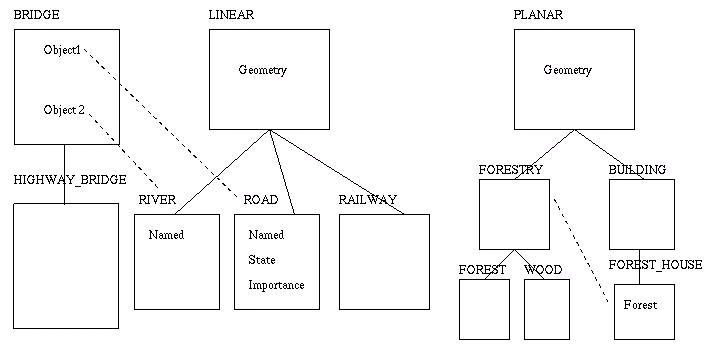
Pic. 3: Object-oriented database schema
E.g. the BRIDGE class consists of all road bridges over rivers. Each bridge has two attributes -- Object1 (a road) and Object2 (a river). Each river (as well as roads and railways) inherits an attribute Geometry(a sequence of (x,y) coordinates) from the class LINEAR. Objects of a class RIVER has no more attributes but Named of the river. In a class ROAD, the attribute State says whether the road is under construction (state=0) or not. The Importance defines a kind of the road:1 stands for highways, 2 for other traffic roads, and3 for the rest(e.g. private ones).
Bridge with Additional Domain Knowledge
Find a description of bridge in terms of attributes of classes road, river, using a predicate common(X,Y). That predicate succeeds if geometries X and Y has a common point.
extract characteristic rule
for
bridge(X,Y):-
object1(X,Z),geometry(Z,G1),
object2(Y,U),geometry(U,G2),
common(G1,G2).
Discrimination of Forests and Woods
Find a difference between forests and woods from the point of view of area. area is the name of set of predicates like area(Geometry,Area).
forest(F) :-
geometry(F,GForest),
area(GForest,Area),
100 < Area.
Relation between Forests and Woods
Find a relation between forests and woods from the point of view of area. area is the name of set of predicates like area(Geometry,Area).
forestOrWood(F,W) :-
geometry(F,GF),area(GF,FA),
geometry(W,GW), area(GW,WA),
WA<GA.
Summary
The query language is quite powerful. It means that even quite complex queries can be expressed. However, the current version of GWiM is incapable to process large amount of data. A solution is discussed in [17].
5. Conclusion
We have presented some approaches for mining spatial data both for relational and object-oriented databases. Although those systems have not reached their maturity yet., nevertheless they represent the first steps that needed to be done.
References
1. Data Mining, Communications of ACM, Vol. 39 No. 11, Nov. 1996.
2. Bancilhon F., Delobel C., Kanellakis P.: Building an Object-Oriented Databases Systems: The story of O2. Morgan Kaufmann 1992.
3. Bigolin N.M., Marsala C.: Fuzzy Spatial OQL for Fuzzy Knowledge Discovery in Databases. In Z.ytkow J.M.,Quafafaou M.(eds.): Principles of Data Mining and Knowledge Discovery. Porc. of 2nd Eur.Symposium, PKDD'98, Nantes, France. LNCS 1510, Springer Verlag 1998.
4. Ester M., Kriegel H.-P., Sander J.: Spatial Data Mining: A Database Approach.In: Proc. of the 5th Int. Symposium on Large Spatial Databases(SSD'97), Berlin. LNCS Vol.1262, pp.47-66, Springer Verlag 1997.
5. Ester M., Frommelt A., Kriegel H.-P., Sander J.: Algorithms for Characterization and Trend Detection in Spatial Databases. In: Proc. of 4th Int. Conf. on Knowledge Discovery and Data Mining (KDD-98).
6. Fayyad, U.M., Piatetski-Shapiro G., Smyth P.: From Data Mining to Knowledge Discovery: An Overview. In: Advances in Knowledge Discovery and Data Mining. AAAI Press/ The MIT Press, Menlo Park, California (1996) 134.
7. Flener P., Popelínský L. Štěpánková: ILP nad Automatic Programming: Towards three approaches. In Wrobel S.(ed.): Proc. of 4th Workshop on Inductive Logic Programming ILP'94, Bad Honeff,Germany, 1994.
8. Grobelnik M.: Induction of Prolog programs with Markus. In Deville Y.(ed.) Proceedings of LOPSTR'93. Workshops in Computing Series, pages 57-63,SpringerVerlag, 1994.
9. K. Koperski, J. Han: Discovery of Spatial Association Rules in Geographic Information Databases. Proceedings of SSD'95, 1995.
10. Han et al.: DMQL: A Data Mining Query Language for Relational Databases. In:ACM-SIGMOD'96 Workshop on Data Mining
11. J. Han, K. Koperski, and N. Stefanovic: GeoMiner: A System Prototype for Spatial Data Mining, Proc. 1997 ACM-SIGMOD Int'l Conf. on Management of Data(SIGMOD'97), Tucson, Arizona, May1997(System prototype demonstration)
12. Imelinski T., Mannila H.: A Database Perspective on Knowledge Discovery. In [1].
13. Lavrač N., Džeroski, Kazakov D., Štěpánková O.: ILPNET repos
itories on WWW: Inductive Logic Programming systems, datasets and bibliography. AI Communications Vol.9, No.4, 1996, pp. 157-206 .14. Koperski K., Han J., Adhikary J.: Mining Knowledge in Geographical Data. Toappear in Comm.of ACM 1998
15. Muggleton S., De Raedt L.: Inductive Logic Programming: Theory And Methods. J. Logic Programming 1994:19,20:629-679. 16. Popeli'nsky' L.: Inductive inference to support object-oriented analysis and design.In: Proc. of 3rd JCKBSE Conference, Smolenice 1998, IOS Press.
17. Popelínský L.: Knowledge Discovery in Spatial Data by Means of ILP. In Z.ytkow J.M., Quafafaou M.(eds.): Principles of Data Mining and Knowledge Discovery. Porc. of 2nd Eur.Symposium, PKDD'98, Nantes, France. LNCS 1510, Springer Verlag 1998.
18. Popelínský L.: Quo vadis, data mining? Sborník konference DATASEM’97, Brno 1997
19. Quinlan J.R.: C4.5: Programs for Machine Learning. Morgan Kaufmann Publ.1992. 19. Shapiro Y.: Algorithmic Program Debugging. MIT Press, 1983.
20. Shapiro, E.: Algorithmic Program Debugging. MIT Press 1983.